
Negative Z Score Table
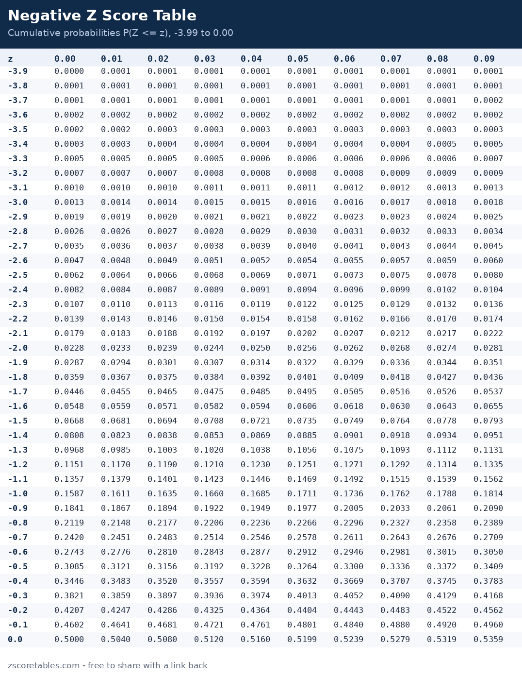
The negative z score table gives the cumulative probability for every z score from −3.99 to 0.00 — the share of the standard normal distribution below that value. Type a z score in the finder and the table jumps straight to your cell with the row and column lit up, or read it manually: row for the first decimal, column for the second.
| z | 0.00 | 0.01 | 0.02 | 0.03 | 0.04 | 0.05 | 0.06 | 0.07 | 0.08 | 0.09 |
|---|---|---|---|---|---|---|---|---|---|---|
| -3.9 | 0.0000 | 0.0001 | 0.0001 | 0.0001 | 0.0001 | 0.0001 | 0.0001 | 0.0001 | 0.0001 | 0.0001 |
| -3.8 | 0.0001 | 0.0001 | 0.0001 | 0.0001 | 0.0001 | 0.0001 | 0.0001 | 0.0001 | 0.0001 | 0.0001 |
| -3.7 | 0.0001 | 0.0001 | 0.0001 | 0.0001 | 0.0001 | 0.0001 | 0.0001 | 0.0001 | 0.0001 | 0.0002 |
| -3.6 | 0.0002 | 0.0002 | 0.0002 | 0.0002 | 0.0002 | 0.0002 | 0.0002 | 0.0002 | 0.0002 | 0.0002 |
| -3.5 | 0.0002 | 0.0002 | 0.0003 | 0.0003 | 0.0003 | 0.0003 | 0.0003 | 0.0003 | 0.0003 | 0.0003 |
| -3.4 | 0.0003 | 0.0003 | 0.0004 | 0.0004 | 0.0004 | 0.0004 | 0.0004 | 0.0004 | 0.0005 | 0.0005 |
| -3.3 | 0.0005 | 0.0005 | 0.0005 | 0.0005 | 0.0006 | 0.0006 | 0.0006 | 0.0006 | 0.0006 | 0.0007 |
| -3.2 | 0.0007 | 0.0007 | 0.0007 | 0.0008 | 0.0008 | 0.0008 | 0.0008 | 0.0009 | 0.0009 | 0.0009 |
| -3.1 | 0.0010 | 0.0010 | 0.0010 | 0.0011 | 0.0011 | 0.0011 | 0.0012 | 0.0012 | 0.0013 | 0.0013 |
| -3.0 | 0.0013 | 0.0014 | 0.0014 | 0.0015 | 0.0015 | 0.0016 | 0.0016 | 0.0017 | 0.0018 | 0.0018 |
| -2.9 | 0.0019 | 0.0019 | 0.0020 | 0.0021 | 0.0021 | 0.0022 | 0.0023 | 0.0023 | 0.0024 | 0.0025 |
| -2.8 | 0.0026 | 0.0026 | 0.0027 | 0.0028 | 0.0029 | 0.0030 | 0.0031 | 0.0032 | 0.0033 | 0.0034 |
| -2.7 | 0.0035 | 0.0036 | 0.0037 | 0.0038 | 0.0039 | 0.0040 | 0.0041 | 0.0043 | 0.0044 | 0.0045 |
| -2.6 | 0.0047 | 0.0048 | 0.0049 | 0.0051 | 0.0052 | 0.0054 | 0.0055 | 0.0057 | 0.0059 | 0.0060 |
| -2.5 | 0.0062 | 0.0064 | 0.0066 | 0.0068 | 0.0069 | 0.0071 | 0.0073 | 0.0075 | 0.0078 | 0.0080 |
| -2.4 | 0.0082 | 0.0084 | 0.0087 | 0.0089 | 0.0091 | 0.0094 | 0.0096 | 0.0099 | 0.0102 | 0.0104 |
| -2.3 | 0.0107 | 0.0110 | 0.0113 | 0.0116 | 0.0119 | 0.0122 | 0.0125 | 0.0129 | 0.0132 | 0.0136 |
| -2.2 | 0.0139 | 0.0143 | 0.0146 | 0.0150 | 0.0154 | 0.0158 | 0.0162 | 0.0166 | 0.0170 | 0.0174 |
| -2.1 | 0.0179 | 0.0183 | 0.0188 | 0.0192 | 0.0197 | 0.0202 | 0.0207 | 0.0212 | 0.0217 | 0.0222 |
| -2.0 | 0.0228 | 0.0233 | 0.0239 | 0.0244 | 0.0250 | 0.0256 | 0.0262 | 0.0268 | 0.0274 | 0.0281 |
| -1.9 | 0.0287 | 0.0294 | 0.0301 | 0.0307 | 0.0314 | 0.0322 | 0.0329 | 0.0336 | 0.0344 | 0.0351 |
| -1.8 | 0.0359 | 0.0367 | 0.0375 | 0.0384 | 0.0392 | 0.0401 | 0.0409 | 0.0418 | 0.0427 | 0.0436 |
| -1.7 | 0.0446 | 0.0455 | 0.0465 | 0.0475 | 0.0485 | 0.0495 | 0.0505 | 0.0516 | 0.0526 | 0.0537 |
| -1.6 | 0.0548 | 0.0559 | 0.0571 | 0.0582 | 0.0594 | 0.0606 | 0.0618 | 0.0630 | 0.0643 | 0.0655 |
| -1.5 | 0.0668 | 0.0681 | 0.0694 | 0.0708 | 0.0721 | 0.0735 | 0.0749 | 0.0764 | 0.0778 | 0.0793 |
| -1.4 | 0.0808 | 0.0823 | 0.0838 | 0.0853 | 0.0869 | 0.0885 | 0.0901 | 0.0918 | 0.0934 | 0.0951 |
| -1.3 | 0.0968 | 0.0985 | 0.1003 | 0.1020 | 0.1038 | 0.1056 | 0.1075 | 0.1093 | 0.1112 | 0.1131 |
| -1.2 | 0.1151 | 0.1170 | 0.1190 | 0.1210 | 0.1230 | 0.1251 | 0.1271 | 0.1292 | 0.1314 | 0.1335 |
| -1.1 | 0.1357 | 0.1379 | 0.1401 | 0.1423 | 0.1446 | 0.1469 | 0.1492 | 0.1515 | 0.1539 | 0.1562 |
| -1.0 | 0.1587 | 0.1611 | 0.1635 | 0.1660 | 0.1685 | 0.1711 | 0.1736 | 0.1762 | 0.1788 | 0.1814 |
| -0.9 | 0.1841 | 0.1867 | 0.1894 | 0.1922 | 0.1949 | 0.1977 | 0.2005 | 0.2033 | 0.2061 | 0.2090 |
| -0.8 | 0.2119 | 0.2148 | 0.2177 | 0.2206 | 0.2236 | 0.2266 | 0.2296 | 0.2327 | 0.2358 | 0.2389 |
| -0.7 | 0.2420 | 0.2451 | 0.2483 | 0.2514 | 0.2546 | 0.2578 | 0.2611 | 0.2643 | 0.2676 | 0.2709 |
| -0.6 | 0.2743 | 0.2776 | 0.2810 | 0.2843 | 0.2877 | 0.2912 | 0.2946 | 0.2981 | 0.3015 | 0.3050 |
| -0.5 | 0.3085 | 0.3121 | 0.3156 | 0.3192 | 0.3228 | 0.3264 | 0.3300 | 0.3336 | 0.3372 | 0.3409 |
| -0.4 | 0.3446 | 0.3483 | 0.3520 | 0.3557 | 0.3594 | 0.3632 | 0.3669 | 0.3707 | 0.3745 | 0.3783 |
| -0.3 | 0.3821 | 0.3859 | 0.3897 | 0.3936 | 0.3974 | 0.4013 | 0.4052 | 0.4090 | 0.4129 | 0.4168 |
| -0.2 | 0.4207 | 0.4247 | 0.4286 | 0.4325 | 0.4364 | 0.4404 | 0.4443 | 0.4483 | 0.4522 | 0.4562 |
| -0.1 | 0.4602 | 0.4641 | 0.4681 | 0.4721 | 0.4761 | 0.4801 | 0.4840 | 0.4880 | 0.4920 | 0.4960 |
| 0.0 | 0.5000 | 0.5040 | 0.5080 | 0.5120 | 0.5160 | 0.5199 | 0.5239 | 0.5279 | 0.5319 | 0.5359 |
Entries are P(Z ≤ z), the area to the left of z. Every entry here is below 0.5000 — that is the built-in check for negative work: a negative z score sits below the mean, so less than half the curve can lie to its left. If your answer for a negative z comes out above 0.5, you have read the positive twin's value instead.
How to use the negative table
- Find the row for the whole number and first decimal place, keeping the minus sign. For z = −1.35, that is row −1.3.
- Find the column for the second decimal place: 0.05.
- Read the meeting point. Row −1.3 and column 0.05 meet at 0.0885, so 8.85% of values lie below z = −1.35.
- Shape the answer. "Above −1.35" is 1 − 0.0885 = 0.9115. "Between −1.35 and the mean" is 0.5000 − 0.0885 = 0.4115. The finder prints every shape at once.
Worked examples
Example 1 — a low test score
A reading test has a mean of 60 and a standard deviation of 8. A student scoring 54 has z = (54 − 60) / 8 = −0.75. The negative table gives Φ(−0.75) = 0.2266: the student scored above only 22.66% of the group — the 23rd percentile, roughly. (The reverse problem also matters: a z of −0.75 with this mean and spread converts back to X = 60 + (−0.75 × 8) = 54.)
Example 2 — the bottom 1% cutoff
Quality teams flag the most extreme low measurements for review. Reading this table backwards, the entry closest to 0.0100 sits at z = −2.33 (0.0099). So about 1% of values fall below z = −2.33, and a measurement there is roughly a once-in-a-hundred event under the model. The precise 1% point is z = −2.326, one of the critical z values.
Example 3 — probability between two negative scores
What share of values falls between z = −2.00 and z = −1.00? Read both ends: Φ(−1.00) = 0.1587 and Φ(−2.00) = 0.0228. Subtract: 0.1587 − 0.0228 = 0.1359, so 13.59% of values lie in that band. The rule never changes: bigger cumulative minus smaller cumulative, whatever the signs.
Example 4 — checking with symmetry
Suppose the negative table is not at hand. Φ(−0.85) can be rebuilt from the positive table: Φ(0.85) = 0.8023, and symmetry gives Φ(−0.85) = 1 − 0.8023 = 0.1977 — exactly what this table prints. Knowing the rule means a positive-only textbook table can still answer every negative question.
Why negative z scores confuse people (and how not to be confused)
A negative z score is not a negative probability, a negative value, or an error. It is simply an address: the minus sign says the value sits below the mean, and the number says by how many standard deviations. A z of −1.35 is the mirror image of +1.35 — same distance, opposite direction. Exam scores below average, temperatures below a seasonal norm, weights below a reference mean: all produce negative z scores, and all are read from this table in exactly the same way as positive ones.
The two genuine traps are these. First, tail direction: for negative z, the "small" answer (the left tail) is the table entry itself, while the "big" answer (everything above it) is 1 minus the entry — the reverse of the pattern students memorise from positive examples. Second, layout mixing: some printed tables list negative z with mean-to-z values instead of cumulative ones, so the same cell position holds a different number (at −1.00: cumulative 0.1587 versus mean-to-z 0.3413). Our standard normal table page shows all three layouts side by side so you can identify which one a question is using. If negative scores themselves are the puzzle, what is a z score explains the sign convention with more examples.
Negative z scores in hypothesis testing
In testing, the negative half of the table does quiet but essential work. A left-tailed test rejects when the statistic falls below a negative critical value: at α = 0.05 the fence is z = −1.645, and at α = 0.01 it is −2.326 — both read straight off this table (0.0500 and 0.0100 in the body). A two-tailed test uses both fences: ±1.96 at 5%, ±2.576 at 1%. This is also where a subtle marking point lives: the p-value of a negative statistic in a left-tailed test is the table entry itself (Φ(−1.84) = 0.0329, significant at 5%), while the same statistic in a two-tailed test must be doubled (0.0658, not significant). Students who memorise "the p-value is the small number" without the tail logic get exactly one of those two right. The critical z values page lists both fences at every common level, and the p-value tool applies the tail logic for you when you want a check.
Frequently asked questions
What does a negative z score mean?
The value is below the mean. The size of the number is the distance in standard deviations: z = −2.00 means two standard deviations below the mean. It says nothing bad by itself — half of all values in any normal distribution have negative z scores.
Can a probability from this table be negative?
No. Probabilities live between 0 and 1. The minus sign belongs to the z score (the position), never to the area. The smallest entries here, near z = −3.99, are about 0.00003.
How do I find the area to the right of a negative z score?
Subtract the table entry from 1. For z = −1.35: 1 − 0.0885 = 0.9115. By symmetry this equals the area to the left of +1.35, which is why the answer is large: most of the curve sits above a below-average point.
Why do some textbooks not print a negative table?
Page space. Symmetry (Φ(−z) = 1 − Φ(z)) lets one positive table do both jobs. We publish both because reading a value directly is faster and less error-prone under pressure.
What z score marks the bottom 5%?
z = −1.645. Reading the table backwards, 0.0500 sits at row −1.6, column 0.045 — between the printed −1.64 (0.0505) and −1.65 (0.0495), and the exact value is −1.645. It is the mirror of the famous 95th-percentile value.
Next steps: the full method is on how to read a z score table, and the mirror values are on the positive z score table.