Positive Z Score Table

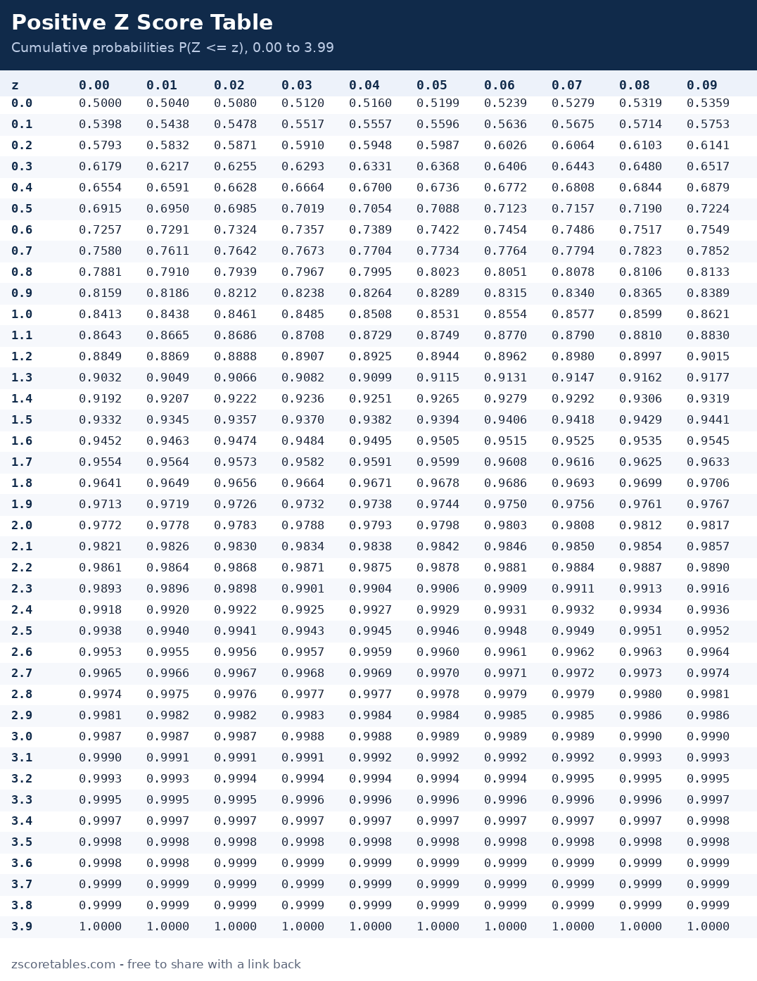
The positive z score table gives the cumulative probability for every z score from 0.00 to 3.99 — the share of the standard normal distribution below that value. Type a z score in the finder and the table jumps to your cell, or read it the textbook way: row for the first decimal, column for the second.

Type a z score or a probability

Area to the left—

Area to the right—

Between mean and z—

Percentile—

Shade:

Area between two z scores:

Positive z score table: cumulative probabilities P(Z ≤ z) from 0.00 to 3.99
z	0.00	0.01	0.02	0.03	0.04	0.05	0.06	0.07	0.08	0.09
0.0	0.5000	0.5040	0.5080	0.5120	0.5160	0.5199	0.5239	0.5279	0.5319	0.5359
0.1	0.5398	0.5438	0.5478	0.5517	0.5557	0.5596	0.5636	0.5675	0.5714	0.5753
0.2	0.5793	0.5832	0.5871	0.5910	0.5948	0.5987	0.6026	0.6064	0.6103	0.6141
0.3	0.6179	0.6217	0.6255	0.6293	0.6331	0.6368	0.6406	0.6443	0.6480	0.6517
0.4	0.6554	0.6591	0.6628	0.6664	0.6700	0.6736	0.6772	0.6808	0.6844	0.6879
0.5	0.6915	0.6950	0.6985	0.7019	0.7054	0.7088	0.7123	0.7157	0.7190	0.7224
0.6	0.7257	0.7291	0.7324	0.7357	0.7389	0.7422	0.7454	0.7486	0.7517	0.7549
0.7	0.7580	0.7611	0.7642	0.7673	0.7704	0.7734	0.7764	0.7794	0.7823	0.7852
0.8	0.7881	0.7910	0.7939	0.7967	0.7995	0.8023	0.8051	0.8078	0.8106	0.8133
0.9	0.8159	0.8186	0.8212	0.8238	0.8264	0.8289	0.8315	0.8340	0.8365	0.8389
1.0	0.8413	0.8438	0.8461	0.8485	0.8508	0.8531	0.8554	0.8577	0.8599	0.8621
1.1	0.8643	0.8665	0.8686	0.8708	0.8729	0.8749	0.8770	0.8790	0.8810	0.8830
1.2	0.8849	0.8869	0.8888	0.8907	0.8925	0.8944	0.8962	0.8980	0.8997	0.9015
1.3	0.9032	0.9049	0.9066	0.9082	0.9099	0.9115	0.9131	0.9147	0.9162	0.9177
1.4	0.9192	0.9207	0.9222	0.9236	0.9251	0.9265	0.9279	0.9292	0.9306	0.9319
1.5	0.9332	0.9345	0.9357	0.9370	0.9382	0.9394	0.9406	0.9418	0.9429	0.9441
1.6	0.9452	0.9463	0.9474	0.9484	0.9495	0.9505	0.9515	0.9525	0.9535	0.9545
1.7	0.9554	0.9564	0.9573	0.9582	0.9591	0.9599	0.9608	0.9616	0.9625	0.9633
1.8	0.9641	0.9649	0.9656	0.9664	0.9671	0.9678	0.9686	0.9693	0.9699	0.9706
1.9	0.9713	0.9719	0.9726	0.9732	0.9738	0.9744	0.9750	0.9756	0.9761	0.9767
2.0	0.9772	0.9778	0.9783	0.9788	0.9793	0.9798	0.9803	0.9808	0.9812	0.9817
2.1	0.9821	0.9826	0.9830	0.9834	0.9838	0.9842	0.9846	0.9850	0.9854	0.9857
2.2	0.9861	0.9864	0.9868	0.9871	0.9875	0.9878	0.9881	0.9884	0.9887	0.9890
2.3	0.9893	0.9896	0.9898	0.9901	0.9904	0.9906	0.9909	0.9911	0.9913	0.9916
2.4	0.9918	0.9920	0.9922	0.9925	0.9927	0.9929	0.9931	0.9932	0.9934	0.9936
2.5	0.9938	0.9940	0.9941	0.9943	0.9945	0.9946	0.9948	0.9949	0.9951	0.9952
2.6	0.9953	0.9955	0.9956	0.9957	0.9959	0.9960	0.9961	0.9962	0.9963	0.9964
2.7	0.9965	0.9966	0.9967	0.9968	0.9969	0.9970	0.9971	0.9972	0.9973	0.9974
2.8	0.9974	0.9975	0.9976	0.9977	0.9977	0.9978	0.9979	0.9979	0.9980	0.9981
2.9	0.9981	0.9982	0.9982	0.9983	0.9984	0.9984	0.9985	0.9985	0.9986	0.9986
3.0	0.9987	0.9987	0.9987	0.9988	0.9988	0.9989	0.9989	0.9989	0.9990	0.9990
3.1	0.9990	0.9991	0.9991	0.9991	0.9992	0.9992	0.9992	0.9992	0.9993	0.9993
3.2	0.9993	0.9993	0.9994	0.9994	0.9994	0.9994	0.9994	0.9995	0.9995	0.9995
3.3	0.9995	0.9995	0.9995	0.9996	0.9996	0.9996	0.9996	0.9996	0.9996	0.9997
3.4	0.9997	0.9997	0.9997	0.9997	0.9997	0.9997	0.9997	0.9997	0.9997	0.9998
3.5	0.9998	0.9998	0.9998	0.9998	0.9998	0.9998	0.9998	0.9998	0.9998	0.9998
3.6	0.9998	0.9998	0.9999	0.9999	0.9999	0.9999	0.9999	0.9999	0.9999	0.9999
3.7	0.9999	0.9999	0.9999	0.9999	0.9999	0.9999	0.9999	0.9999	0.9999	0.9999
3.8	0.9999	0.9999	0.9999	0.9999	0.9999	0.9999	0.9999	0.9999	0.9999	0.9999
3.9	1.0000	1.0000	1.0000	1.0000	1.0000	1.0000	1.0000	1.0000	1.0000	1.0000

Entries are P(Z ≤ z), the area to the left of z. Because every positive z sits above the mean, every entry here is above 0.5000 — a useful sanity check: if a positive-table answer ever comes out below 0.5, you are reading the wrong table or the wrong layout.

Download PDF Download PNG image Download CSV

How to use the positive table

Find the row for the whole number and first decimal place of your z score. For z = 0.56, that is row 0.5.
Find the column for the second decimal place. For 0.56, that is column 0.06.
Read the meeting point. Row 0.5 and column 0.06 meet at 0.7123, so 71.23% of values lie below z = 0.56.
Shape the answer to the question. "Above 0.56" means 1 − 0.7123 = 0.2877. "Between the mean and 0.56" means 0.7123 − 0.5000 = 0.2123. The finder above prints all of these at once.

Worked examples

Example 1 — an exam score in the top slice

A class exam has a mean of 70 and a standard deviation of 10. Sara scores 85, so her z score is (85 − 70) / 10 = 1.50. The positive table gives Φ(1.50) = 0.9332: Sara outscored 93.32% of the class, which puts her in roughly the top 6.7% (1 − 0.9332 = 0.0668).

Example 2 — height percentile

Adult heights in a population average 170 cm with a standard deviation of 7 cm. A man who is 182 cm tall has z = (182 − 170) / 7 = 1.71. The table reads 0.9564, so he is taller than 95.64% of the population — the 96th percentile, roughly.

Example 3 — the area between the mean and z = 1.09

Some textbooks ask for the area between the mean and a z score instead of the area to the left. Read the cumulative value first: Φ(1.09) = 0.8621. The mean sits at 0.5000, so the slice between them is 0.8621 − 0.5000 = 0.3621. This is exactly the number a mean-to-z table would print directly — the standard normal table page lets you flip this site's tables into that layout.

Example 4 — a two-tailed test at z = 1.84

A researcher computes a test statistic of z = 1.84. The table gives 0.9671 to the left, so one tail beyond 1.84 holds 1 − 0.9671 = 0.0329. A two-tailed test counts both extremes: p = 2 × 0.0329 = 0.0658, which is not significant at the 0.05 level. Doubling the wrong number — the cumulative entry itself — is the classic error here: 2 × 0.9671 is greater than 1, and a probability never is.

Why the positive table is the one most people print

Because of symmetry, the positive half of the table secretly contains the whole distribution. The area to the left of any negative z equals the area to the right of its positive twin: Φ(−1.25) = 1 − Φ(1.25) = 1 − 0.8944 = 0.1056. That is why so many textbooks print only this table — one page does every job once you know the symmetry rule. We still publish a full negative z score table, because reading a value directly beats doing a subtraction when you are tired, rushed, or sitting an exam.

The positive table is also where the famous critical values live: 1.645 cuts off the top 5%, 1.96 cuts off the top 2.5%, and 2.576 cuts off the top 0.5%. If you are working with confidence intervals rather than single lookups, the confidence intervals page starts from those three values and shows how to find the z for any other level.

Reading between the cells: interpolation

The printed grid steps in hundredths, but real z scores land where they like. The most famous case is 1.645 — the 95th-percentile value — which sits exactly halfway between the 1.64 cell (0.9495) and the 1.65 cell (0.9505). When a value falls between cells, the honest options are three: report the nearer cell and say so; interpolate linearly, taking the fraction of the gap (halfway between 0.9495 and 0.9505 is 0.9500 — here the interpolation happens to be exact); or use a calculator that evaluates the distribution directly. The finder at the top of this page is in the third category, which is why typing 1.645 returns exactly 0.9500 instead of a neighbour. In exams, follow your board's convention — most accept the nearest cell, and critical-value questions are usually set on values the grid holds exactly, like 1.96. What you should never do is round the z score itself to fit the grid without noticing: rounding 1.645 to 1.6 changes the probability to 0.9452, an error five times larger than the one interpolation exists to fix.

positive z score table image with cumulative probabilities from 0.00 to 3.99 — The positive z score table as an image — free to share with a link back. Values are generated from the same source as the interactive table above.

Frequently asked questions

What does the positive z score table tell me?

For any positive z score, it tells you the proportion of the standard normal distribution that lies below it (to its left). Multiply by 100 to read it as a percentage or a percentile: z = 1.00 → 0.8413 → the 84.13th percentile.

Can I use the positive table for a negative z score?

Yes, with the symmetry rule: look up the positive version, then subtract from 1. Φ(−0.85) = 1 − Φ(0.85) = 1 − 0.8023 = 0.1977. Or use our negative table and read the answer directly.

Why does the positive table start at 0.5000?

Because z = 0 is the mean itself, and exactly half of a symmetric distribution lies below its mean. Every step to the right adds area, which is why the entries climb from 0.5000 towards 1.0000 as z grows.

What is the largest value in the positive table?

At z = 3.99 the cumulative probability is 0.99997, which rounds to 1.0000 at four decimal places. Beyond about z = 3.5 the remaining tail is smaller than 0.0003, so for practical purposes almost nothing lies further out — values that extreme are usually flagged as outliers.

Is this the same as Table A in AP Statistics?

Yes. AP's Table A is the cumulative standard normal table: same rows, same columns, same entries. This page adds a finder and colour highlighting on top of the identical numbers.

Next steps: learn the full reading method on how to read a z score table, or test yourself with the practice problems.